a. 1: Description
For this session, we will be working with data compiled from eBird, specifically for two hotspots in Port Aransas: the Leonabelle Turnbull Birding Sanctuary CTC 057 and the Port Aransas Jetty and Beach CTC 058. I have downloaded, compiled, and processed the individual text files to give you a clean slate. I have also assigned broad and fine groups to each bird species in a separate dataset.
b. 1: Data
The dataset called ‘birds_historic_processed.csv’ can be downloaded here.
The dataset called ‘birds_historic_processed_groups_assigned.csv’ can be downloaded here.
c. 1: Tasks
I. Read in the two datasets above. Then, using the “birds_historic_processed.csv” dataset, perform the following steps: 1) determine the total number of species observed each week (across all months and years) and across the two datasets as well as the mean effort expended 2) calculate the species richness per unit effort 2) plot the average species richness per unit effort for each year at each location
library(dplyr)
library(ggplot2)
library(forcats)
bird.data.processed <- read.csv(file = "data/birds_historic_processed.csv")

bird.data.effort <- bird.data.processed %>%
  group_by(year, month, week, location) %>%
  summarize(sprich = sum(presvsabs), effort = mean(effort)) %>%
  mutate(sprich_count = sprich/effort) %>%
  ungroup() %>%
  group_by(location, year) %>%
  summarize(avg_sprich_count = mean(sprich_count),
            sd_sprich_count = sd(sprich_count),
            se_sprich_count = sd_sprich_count/sqrt(n()))

sprichplot <- ggplot(data = bird.data.effort, aes(x = year, y = avg_sprich_count, color = location, group = location)) +
  geom_line() +
  geom_pointrange(aes(x = year, y = avg_sprich_count,
                      ymin = avg_sprich_count-se_sprich_count,
                      ymax = avg_sprich_count+se_sprich_count)) +
  scale_color_manual(values = c("darkviolet",
                                "goldenrod")) +
  theme_classic() +
  ylab("Mean species richness per unit effort") +
  xlab("Year") +
  theme(legend.position = "top",
        legend.title=element_blank())
sprichplot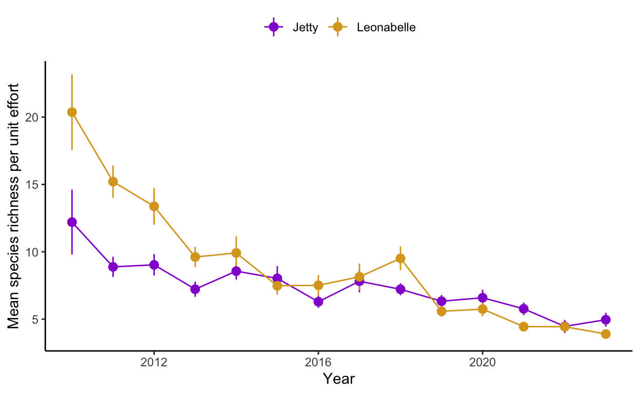
- Join the bird dataset with the group assignments. Then, calculate the total occurrence of each species each year across the two locations for the following three groups: waterbirds, shorebirds, and seabirds. With the resulting data, plot the species-specific abundances at the two locations using box- or violin plots, choosing an intuitive order on the x- or y-axis.
group.assignments <- read.csv(file = "data/birds_historic_processed_groups_assigned.csv")

birds.processed.groups <- bird.data.processed %>%
  left_join(group.assignments)

waterbird.abundance <- birds.processed.groups %>%
  filter(group == "waterbirds") %>%
  group_by(species, location, year) %>%
  summarize(sum.occ = sum(occurrence))

waterbird.abundance.plot <- ggplot(waterbird.abundance, aes(x = fct_reorder(species, -sum.occ, .fun = mean), y = sum.occ)) +
  geom_boxplot(aes(fill = location)) +
  facet_grid(location~., scales = "free") +
  theme_bw() +
  theme(axis.text.x = element_text(angle = 45, hjust = 1)) +
  scale_fill_manual(values = c("darkviolet",
                                "goldenrod")) +
  xlab("")
waterbird.abundance.plot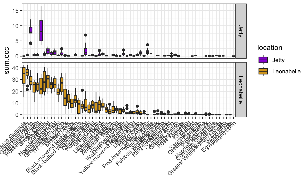
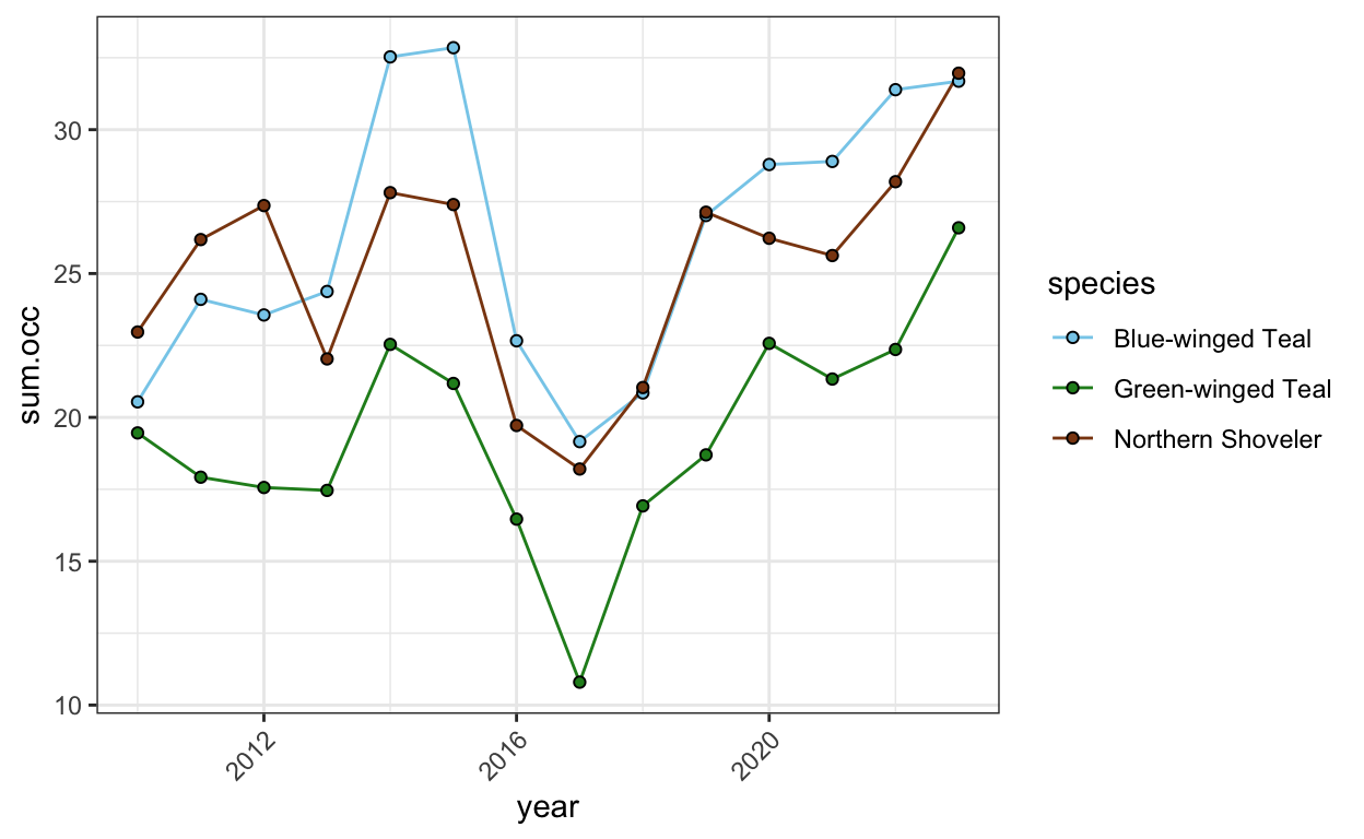
- Find and plot the occurrences of the three most abundant ducks, plovers, and sandpipers at Leonabelle over the examined years.
ducks <- birds.processed.groups %>%
  filter(group2 == "ducks",
         location == "Leonabelle") %>%
  group_by(species, year) %>%
  summarize(sum.occ = sum(occurrence)) %>%
  arrange(fct_reorder(species, -sum.occ, .fun = mean)) %>%
  filter(species %in% c("Blue-winged Teal", "Northern Shoveler", "Green-winged Teal"))

duck.abundance.plot <- ggplot(ducks, aes(x = year, y = sum.occ, group = species)) +
  geom_line(aes(color = species)) +
  geom_point(aes(fill = species), shape = 21) +
  theme_bw() +
  theme(axis.text.x = element_text(angle = 45, hjust = 1)) +
  scale_color_manual(values = c("skyblue",
                               "forestgreen",
                               "chocolate4")) +
  scale_fill_manual(values = c("skyblue",
                                "forestgreen",
                                "chocolate4"))

duck.abundance.plot