Session 6: Functional trait based analyses

This session introduces trait-based analyses as means to analyze communities under the consideration of ecological differences.

a. 6: Exercises

• Start by loading the following packages (remember that you may have to install some of them):

library(tidyverse)
library(fishualize)
library(patchwork)
library(vegan)
library(FD)
library(patchwork)
library(ggformula)

Part I: reef fish traits

Data wrangling:

• We will first work with a reef fish dataset that was used for trait-based analyses in Brandl et al. 2016 (Ecosphere). The trait data are here and the site data, which contains biomass calculations for each community, are here, which we will call “sites”. Load the data into your environment and then use the “column_to_rownames” function to turn the “Species” column (trait dataset) into your rownames.

• For the sites dataset, remove the year column from the dataset and then use the “column_to_rowname” function again, this time for the “site” column. Then turn the sites data.frame into a matrix using the “as.matrix” function.

• Finally, check that the rownames of the trait dataset match the column names of the sites dataset

traits = read.csv(file = "data/traits.csv")
sites = read.csv(file = "data/sites.csv")

traits1 <- traits %>%  
  mutate(Diet = as.factor(Diet),
         Habitat = as.factor(Habitat),
         Territorial = as.factor(Territorial),
         Sizeclass = as.factor(Sizeclass)) %>%
    column_to_rownames("Species")

sites1 <- sites %>%
  select(-year) %>%
  column_to_rownames("site") %>%
  as.matrix()

rownames(traits1) == colnames(sites1)

  [1] TRUE TRUE TRUE TRUE TRUE TRUE TRUE TRUE TRUE TRUE TRUE TRUE TRUE
 [14] TRUE TRUE TRUE TRUE TRUE TRUE TRUE TRUE TRUE TRUE TRUE TRUE TRUE
 [27] TRUE TRUE TRUE TRUE TRUE TRUE TRUE TRUE TRUE TRUE TRUE TRUE TRUE
 [40] TRUE TRUE TRUE TRUE TRUE TRUE TRUE TRUE TRUE TRUE TRUE TRUE TRUE
 [53] TRUE TRUE TRUE TRUE TRUE TRUE TRUE TRUE TRUE TRUE TRUE TRUE TRUE
 [66] TRUE TRUE TRUE TRUE TRUE TRUE TRUE TRUE TRUE TRUE TRUE TRUE TRUE
 [79] TRUE TRUE TRUE TRUE TRUE TRUE TRUE TRUE TRUE TRUE TRUE TRUE TRUE
 [92] TRUE TRUE TRUE TRUE TRUE TRUE TRUE TRUE TRUE TRUE TRUE TRUE TRUE
[105] TRUE TRUE TRUE TRUE TRUE TRUE TRUE TRUE TRUE TRUE TRUE TRUE TRUE
[118] TRUE TRUE TRUE TRUE TRUE TRUE TRUE TRUE TRUE TRUE TRUE TRUE TRUE
[131] TRUE TRUE TRUE TRUE TRUE TRUE TRUE TRUE TRUE TRUE TRUE TRUE TRUE
[144] TRUE TRUE TRUE TRUE TRUE TRUE TRUE TRUE TRUE TRUE TRUE TRUE TRUE
[157] TRUE TRUE TRUE TRUE TRUE TRUE TRUE TRUE TRUE TRUE TRUE TRUE TRUE
[170] TRUE TRUE TRUE TRUE TRUE TRUE TRUE TRUE TRUE TRUE TRUE TRUE TRUE
[183] TRUE TRUE TRUE TRUE TRUE TRUE TRUE TRUE TRUE TRUE TRUE TRUE TRUE
[196] TRUE TRUE TRUE TRUE TRUE TRUE TRUE TRUE TRUE TRUE TRUE TRUE TRUE
[209] TRUE TRUE TRUE TRUE TRUE TRUE TRUE TRUE TRUE TRUE TRUE TRUE TRUE
[222] TRUE TRUE TRUE TRUE TRUE TRUE TRUE TRUE TRUE TRUE TRUE TRUE TRUE
[235] TRUE TRUE TRUE TRUE TRUE TRUE TRUE TRUE TRUE TRUE TRUE TRUE TRUE
[248] TRUE TRUE TRUE TRUE TRUE TRUE TRUE TRUE TRUE TRUE TRUE TRUE TRUE
[261] TRUE TRUE TRUE TRUE TRUE TRUE TRUE TRUE TRUE TRUE TRUE TRUE TRUE

Running FD:

• To calculate the most common functional indices, we will use the dbFD function. Specify the traits dataset and the sites dataset as the two inputs, choose a correction for negative eigenvalues (usually cailliez or lingoes), and make sure to specify “print.pco = TRUE”.

• Pull the number of species (nbsp), functional richness (FRic), functional evenness (FEve), and functional dispersion (FDis) values into a new dataset that also has your sites and the year (from the original sites dataset)

calc <- dbFD(x = traits1, a = sites1, corr = "lingoes", print.pco = T)

Species x species distance matrix was not Euclidean. Lingoes correction was applied. 
FRic: Only categorical and/or ordinal trait(s) present in 'x'. FRic was measured as the number of unique trait combinations, NOT as the convex hull volume. 
FDiv: Cannot be computed when only categorical and/or ordinal trait(s) present in 'x'. 

functional_metrics <- sites %>%
  select(site, year) %>%
  bind_cols(calc$nbsp, calc$FRic, calc$FEve, calc$FDis) %>%
  rename("Spric" = "...3",
    "FRichness" = "...4",
         "FEveness" = "...5",
         "FDispersion" = "...6")

Plotting:

• Plot species richness against functional richness, fitting a line that suggests the best fit to the data

• Plot the four indices in 2011 and 2015 using boxplots, violins, or similar

• Plot the functional space across the two years, calling on the “x.axes” column in the output of the dbFD function

spric_fric <- ggplot(functional_metrics, aes(x = Spric, y = FRichness)) +
  geom_point(color = "sienna2") +
  geom_smooth(method = "lm", formula = y ~ poly(x, 2), color = "sienna2", fill = "sienna4") +
  theme_classic() +
  ylab("Functional richness") +
  xlab("Species richness")
spric_fric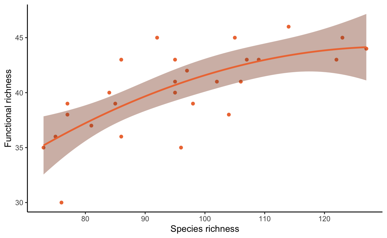

functional_metrics_long <- functional_metrics %>%
  pivot_longer(cols = 3:6, names_to = "metric", values_to = "value")
  
diversity_plots <- ggplot(functional_metrics_long, aes(x = as.factor(year), y = value, fill = as.factor(year))) +
  geom_boxplot() +
  facet_wrap(.~metric, scales = "free") +
  scale_fill_manual(values = c("sienna2", "steelblue")) +
  theme_classic() +
  xlab("Year") +
  ylab("") +
  theme(legend.position = "none")
diversity_plots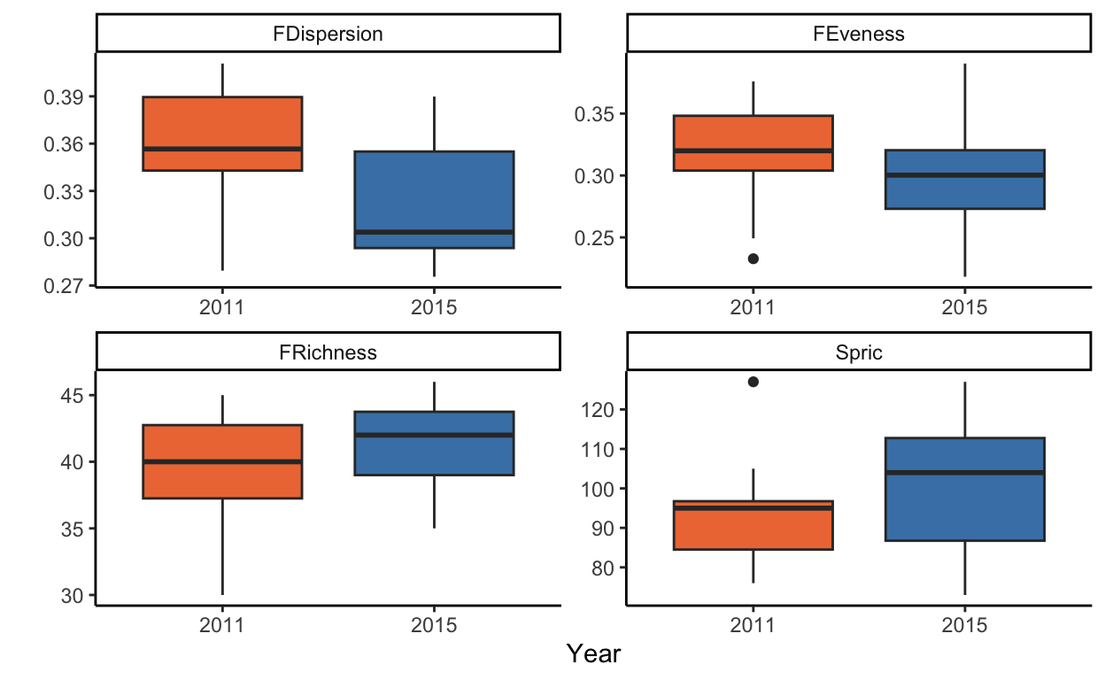

### plot functional space

species.coords <- data.frame(calc$x.axes) %>%
  select(A1, A2) %>%
  mutate(species = rownames(.)) %>%
  mutate(A1 = round(A1, 4),
         A2 = round(A2, 4))

sites.coords <- sites %>%
  pivot_longer(cols = 3:275, names_to = "species", values_to = "biomass") %>%
  inner_join(species.coords) %>%
  filter(biomass > 0) %>%
  group_by(site, year, A1, A2) %>%
  summarize(biomass = sum(biomass))
  
functional.space <- ggplot(sites.coords, aes(x = A1, y = A2, fill = as.factor(year))) +
  geom_point(aes(size = biomass*10), shape = 21, alpha = 0.3) +
  facet_wrap(. ~ year) +
  scale_fill_manual(values = c("sienna2", "steelblue")) +
  theme_classic() +
  xlab("Axis1") +
  ylab("Axis2") +
  theme(legend.position = "none")
functional.space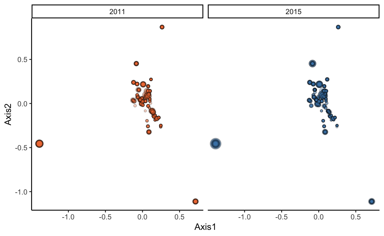

Part II: estuarine fish data

• Download the datasets that contain the traits: here) and the community data: here and read them into your R environment

• Follow the steps above to calculate functional richness, evenness, dispersion, and diversity and plot them across the two communities (the bridge and the channel)

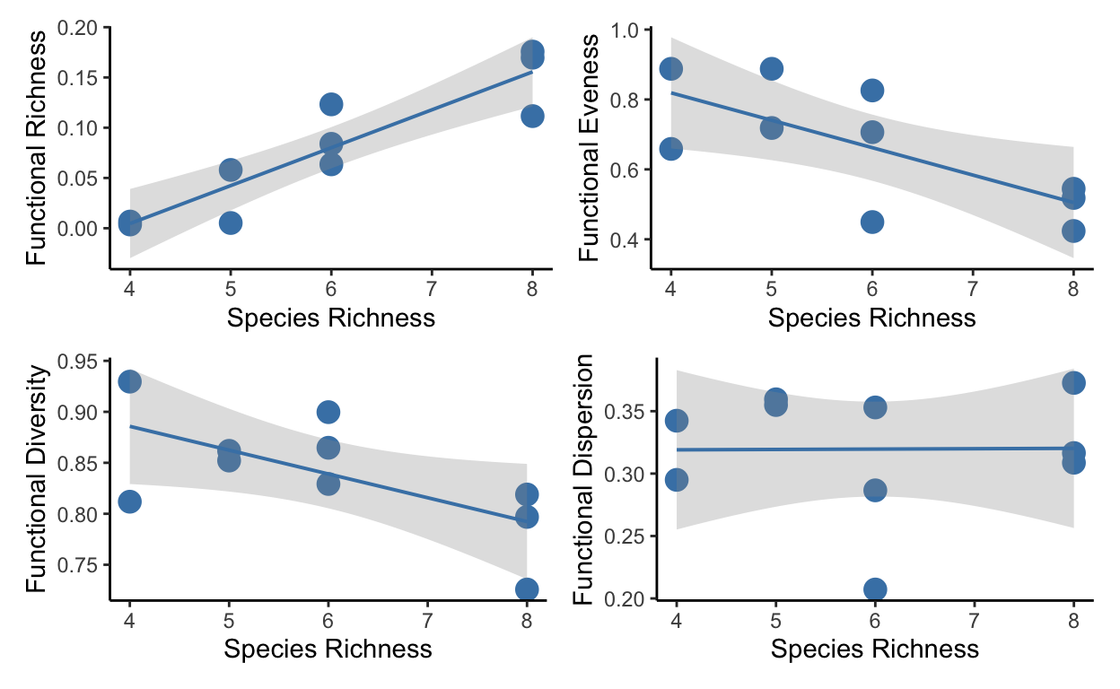
• Plot the relationship between the functional indices and species richness in four scatterplots

Hints:

• make sure your trait lists and community lists match each other, including the alphabetical order. The arrange function will help with this.

• remove any species from the community dataset that do not have a clear taxonomic identity, as they cannot be assigned traits (e.g. larvae)

• make sure your traits are factors, not characters

### TRAIT COMPOSITION IN ESTUARINE FISHES

library(tidyverse)
library(fishualize)
library(patchwork)
library(vegan)
library(FD)
library(patchwork)
library(ggformula)

#reading in community dataset

#We convert each of the trait variables to factors We also need to ensure the order of the trait dataset matches EXACTLY the order of the community composition dataset.

#To do do, we will simply arrange both the order of the trait dataset and the community composition dataset in alphabetical order

fish_traits <- read.csv("data/fish_lab/traits_ed.csv", header = T) %>%
  arrange(Name) %>%
  column_to_rownames("Name") %>%
  mutate_if(is.character,as.factor)

#reading in community composition dataset

# First, we will remove the Leptocephalus.larvae and the Larvae species, as we can not reliably ascribe traits to these taxa. Next, we create a unique ID to be used for the rownames by pasteing the Site and Seine number. Last, we rename the two species that are misspelled, as in the trait dataset they are spelled correctly and we need these to match

community.comp <- read.csv(file = "data/fish_lab/communities.csv") %>%
  select(-Leptocephalus.larvae, -Larvae) %>%
  mutate(ID = paste0(Site, "_", Seine)) %>%
  select(-Seine, -Site) %>%
  column_to_rownames("ID") %>%
  select(order(colnames(.))) %>%
  as.matrix()

#checking the rownames match the column names
rownames(fish_traits) == colnames(community.comp)

 [1] TRUE TRUE TRUE TRUE TRUE TRUE TRUE TRUE TRUE TRUE TRUE TRUE TRUE
[14] TRUE TRUE TRUE TRUE

#############################################################################################################################
###   Now calculating a suite of functional trait metrics for our community using the dbFD function from the FD package   ###
#############################################################################################################################

#functional trait calculation
calc <- dbFD(fish_traits, community.comp, corr = "cailliez")

Species x species distance matrix was not Euclidean. Cailliez correction was applied. 
FRic: Dimensionality reduction was required. The last 12 PCoA axes (out of 15 in total) were removed. 

FRic: Quality of the reduced-space representation (based on corrected distance matrix) = 0.6853169 

functional_metrics <- bind_cols(calc$FRic, calc$FEve, calc$FDiv, calc$FDis) %>%
  rename("FRichness" = "...1",
         "FEveness" = "...2",
         "FDiversity" = "...3",
         "FDispersion" = "...4") %>%
  mutate(Site = c(rep("Bridge", 5), rep("Channel", 5)),
         ID = paste0(Site, "_", rep(1:5, 2)))

rownames(functional_metrics) <- functional_metrics$ID



#Now plotting our different metrics to explore how these functional traits relate to structured vs open habitats

plot_richness <- ggplot(data = functional_metrics, aes(x = Site, y = FRichness, color = Site, fill = Site)) +
  stat_summary(fun.data=function(x){mean_cl_normal(x, conf.int=.683)}, geom="linerange", 
               linewidth=1, alpha=0.7) +
  stat_summary(fun.y=mean, geom="point", pch=21, size=5, color = "black") +
  geom_jitter(width = 0.1, size = 2, pch = 21, color = "black") +
  theme_classic() +
  scale_fill_manual(values = c("wheat4", "skyblue3")) +
  scale_color_manual(values = c("wheat4", "skyblue3")) +
  theme(legend.position = "none") +
  xlab("")

plot_eveness <- ggplot(data = functional_metrics, aes(x = Site, y = FEveness, color = Site, fill = Site)) +
  stat_summary(fun.data=function(x){mean_cl_normal(x, conf.int=.683)}, geom="linerange", 
               linewidth=1, alpha=0.7) +
  stat_summary(fun.y=mean, geom="point", pch=21, size=5, color = "black") +
  geom_jitter(width = 0.1, size = 2, pch = 21, color = "black") +
  theme_classic() +
  scale_fill_manual(values = c("wheat4", "skyblue3")) +
  scale_color_manual(values = c("wheat4", "skyblue3")) +
  theme(legend.position = "none") +
  xlab("")

plot_diversity <- ggplot(data = functional_metrics, aes(x = Site, y = FDiversity, color = Site, fill = Site)) +
  stat_summary(fun.data=function(x){mean_cl_normal(x, conf.int=.683)}, geom="linerange", 
               linewidth=1, alpha=0.7) +
  stat_summary(fun.y=mean, geom="point", pch=21, size=5, color = "black") +
  geom_jitter(width = 0.1, size = 2, pch = 21, color = "black") +
  theme_classic() +
  scale_fill_manual(values = c("wheat4", "skyblue3")) +
  scale_color_manual(values = c("wheat4", "skyblue3")) +
  theme(legend.position = "none") +
  xlab("")

plot_dispersion <- ggplot(data = functional_metrics, aes(x = Site, y = FDispersion, color = Site, fill = Site)) +
  stat_summary(fun.data=function(x){mean_cl_normal(x, conf.int=.683)}, geom="linerange", 
               linewidth=1, alpha=0.7) +
  stat_summary(fun.y=mean, geom="point", pch=21, size=5) +
  stat_summary(fun.y=mean, geom="point", pch=21, size=5, color = "black") +
  geom_jitter(width = 0.1, size = 2, pch = 21, color = "black") +
  theme_classic() +
  scale_fill_manual(values = c("wheat4", "skyblue3")) +
  scale_color_manual(values = c("wheat4", "skyblue3")) +
  theme(legend.position = "none") +
  xlab("")


fdplots <- (plot_richness | plot_eveness) / (plot_diversity | plot_dispersion)
fdplots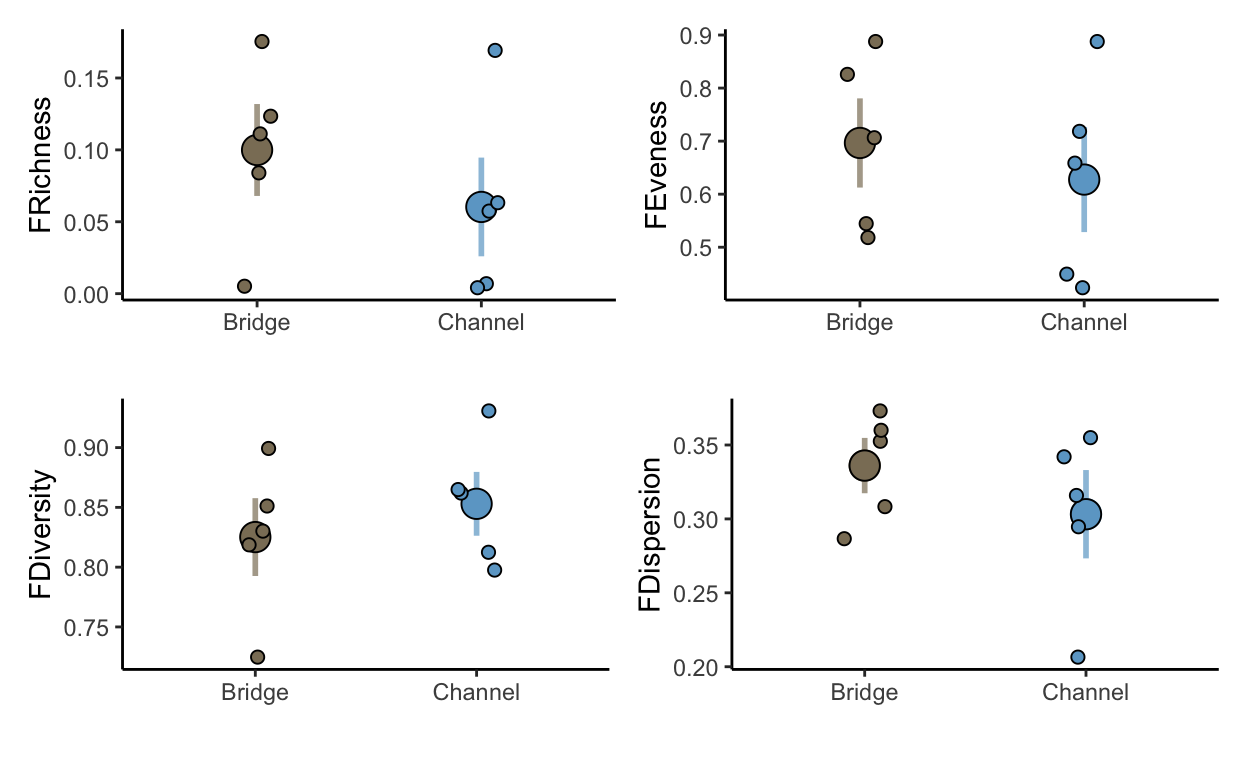

#########################################################################
###  Last, well explore how these metrics relate to species richness  ###
#########################################################################

#species richness and abundance per seine

com.str <- read.csv(file = "data/fish_lab/communities.csv") %>%
  pivot_longer(cols = -c("Site", "Seine")) %>%
  filter(!name %in% c("Leptocephalus.larvae", "Larvae")) %>%
  group_by(Site, Seine) %>%
  filter(value > 0) %>%
  summarize(sprich = n_distinct(name), abundance = sum(value)) %>%
  mutate(ID = paste0(Site, "_", Seine))

merged_data <- left_join(com.str, functional_metrics)

a.1 <- ggplot(merged_data, aes(x = sprich, y = FRichness)) +
  geom_point(size = 4, color = "steelblue") +
  theme_classic() +
  theme(legend.position = "none") +
  geom_lm(interval = "confidence", color = "steelblue") +
  xlab("Species Richness") +
  ylab("Functional Richness")

b.1 <- ggplot(merged_data, aes(x = sprich, y = FEveness)) +
  geom_point(size = 4, color = "steelblue") +
  theme_classic() +
  theme(legend.position = "none") +
  geom_lm(interval = "confidence", color = "steelblue") +
  xlab("Species Richness") +
  ylab("Functional Eveness")

c.1 <- ggplot(merged_data, aes(x = sprich, y = FDiversity)) +
  geom_point(size = 4, color = "steelblue") +
  theme_classic() +
  theme(legend.position = "none") +
  geom_lm(interval = "confidence", color = "steelblue") +
  xlab("Species Richness") +
  ylab("Functional Diversity")

d.1 <- ggplot(merged_data, aes(x = sprich, y = FDispersion)) +
  geom_point(size = 4, color = "steelblue") +
  theme_classic() +
  theme(legend.position = "none") +
  geom_lm(interval = "confidence", color = "steelblue") +
  xlab("Species Richness") +
  ylab("Functional Dispersion")


plot.relat <- (a.1 | b.1) / (c.1 | d.1)
plot.relat