a. 1: Description
For this lab, we will be working with the data you collected during the previous two fish labs. Specifically, we will use three different datasets to create data visualizations that you can use for your presentations. It is also a precursor to next weeks functional trait lab.
b. 1: Data
The dataset called ‘communities’ can be downloaded here. It describes the counts of different fish species collected during ten seine net drags in two habitats (five each). The “bridge” habitat was characterized by the availability of human made structure (the bridge pillars), while the “channel” habitat was characterized by natural, unstructured habitat.
The dataset called ‘guts’ can be downloaded here. It has the presence (1) and absence (0) of six different prey categories in a variety of fishes from 10 species found in the community dataset.
The dataset called ‘morphometrics’ can be downloaded here. It contains morphometric measurements of individuals across several different species found in the community dataset.
c. 1: Tasks
I. Read in the communities dataset. Then perform the following actions:
• examine the community composition of estuarine fishes at the bridge and channel sites using a Principal Component Analyses based on Hellinger transformed abundances of species across seines.
• bring the data to long format, calculate the species richness and total abundance of fishes in each seine, and plot the two metrics (species richness and abundance) across the two sites (bridge and channel).
library(tidyverse)
library(fishualize)
library(patchwork)
library(vegan)

# community composition

community.comp <- read.csv(file = "data/fish_lab/communities.csv")

comp.meta <- community.comp[1:2]

comp.raw.hell <- decostand(community.comp[-c(1:2)], method = "hellinger")

comp.pca <- rda(comp.raw.hell, scale = F)
sum.pca <- summary(comp.pca)

comp_scores <- as.data.frame(sum.pca$sites) %>%
  mutate(Assemblage = rownames(.)) %>%
  bind_cols(comp.meta)

comp_vectors <- as.data.frame(sum.pca$species) %>%
  mutate(vectors = rownames(.))

comp_hulls <- comp_scores %>%
  group_by(Site) %>%
  slice(chull(PC1, PC2))

comp.plot <- ggplot() +
  geom_point(data = comp_scores, aes(x = PC1, y = PC2, color = Site), size = 2) +
  geom_polygon(data = comp_hulls, aes(x = PC1, PC2, fill = Site), alpha = 0.5) +
  geom_segment(data = comp_vectors, aes(x = 0, xend = PC1,
                                           y = 0, yend = PC2), lwd = 0.1) +
  geom_label(data = comp_vectors, aes(x = PC1, y = PC2, label = vectors), size = 2) +
  scale_fill_fish_d(option = "Trimma_lantana", alpha = 0.5) +
  scale_color_fish_d(option = "Trimma_lantana") +
  theme_bw() +
  xlab("PC1 (34.9%)") +
  ylab("PC2 (31.2%)")
comp.plot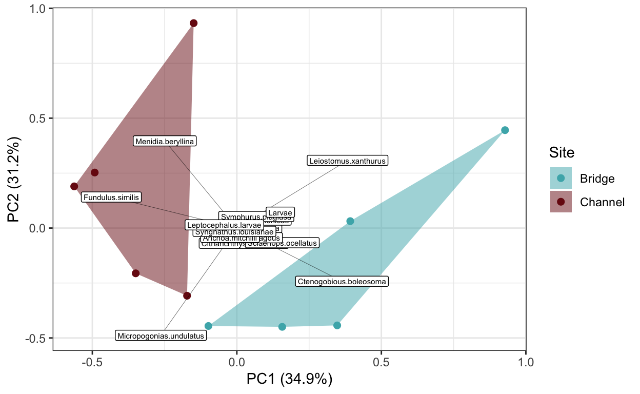
# community data
community <- read.csv(file = "data/fish_lab/communities.csv") %>%
  pivot_longer(cols = 3:21, names_to = "Species.ID", values_to = "count")

# species richness and abundance per seine
com.str <- community %>%
  group_by(Site, Seine) %>%
  filter(count > 0) %>%
  summarize(sprich = n_distinct(Species.ID), abundance = sum(count))

sprich.plot <- ggplot(com.str, aes(x = Site, y = sprich, fill = Site, color = Site)) +
  stat_summary(fun.data=function(x){mean_cl_normal(x, conf.int=.683)}, geom="errorbar",
               width=0.03, alpha=0.7) +
  stat_summary(fun.y=mean, geom="point", pch=21, size=3) +
  geom_jitter(shape = 21, width = 0.1, height = 0) +
  scale_fill_fish_d(option = "Trimma_lantana", alpha = 0.5) +
  scale_color_fish_d(option = "Trimma_lantana") +
  theme_classic() +
  ylab("Species richness") +
  xlab("")


abu.plot <- ggplot(com.str, aes(x = Site, y = abundance, fill = Site, color = Site)) +
  stat_summary(fun.data=function(x){mean_cl_normal(x, conf.int=.683)}, geom="errorbar",
               width=0.03, alpha=0.7) +
  stat_summary(fun.y=mean, geom="point", pch=21, size=3) +
  geom_jitter(shape = 21, width = 0.1, height = 0) +
  scale_fill_fish_d(option = "Trimma_lantana", alpha = 0.5) +
  scale_color_fish_d(option = "Trimma_lantana") +
  theme_classic() +
  ylab("Abundance") +
  xlab("")

structure.plots <- sprich.plot + abu.plot + plot_annotation(tag_levels = 'a') + plot_layout(guides = "collect")

structure.plots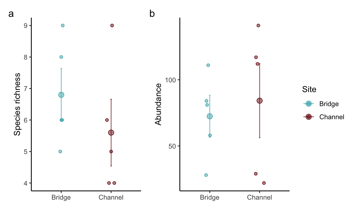
- Read in the guts dataset. Then perform the following actions:
• calculate the percentual occurrence of different prey items in the guts of each species. To do so, you will need to add up the number of individuals examined in each species, as well as the number of times a prey item was discovered in this species, and then divide the latter by the former.
• plot the percent occurrence of prey items across the ten species in a barchart, using axes and colors to delineate both fish species and their prey.
# gut content % occurrence

guts <- read.csv(file = "data/fish_lab/guts.csv") %>%
  group_by(Species.ID) %>%
  mutate(total_n = n_distinct(Individual)) %>%
  pivot_longer(cols = c(5:10), names_to = "prey", values_to = "pres") %>%
  group_by(Species.ID, prey, total_n) %>%
  summarize(occurrence = sum(pres)) %>%
  mutate(percent_occurrence = occurrence/total_n*100)

percent_plot <- ggplot(guts, aes(x = percent_occurrence, y = Species.ID)) +
  geom_bar(aes(fill = prey, color = prey), stat = "identity", position = position_dodge(width = 1)) +
  geom_label(aes(x = 105, y = Species.ID, label = total_n), size = 3)+
  scale_fill_fish_d(option = "Trimma_lantana", alpha = 0.5) +
  scale_color_fish_d(option = "Trimma_lantana") +
  theme_classic() +
  ylab("") +
  xlab("% occurrence") +
  theme(axis.text.y = element_text(face = "italic"),
        legend.title = element_blank())
percent_plot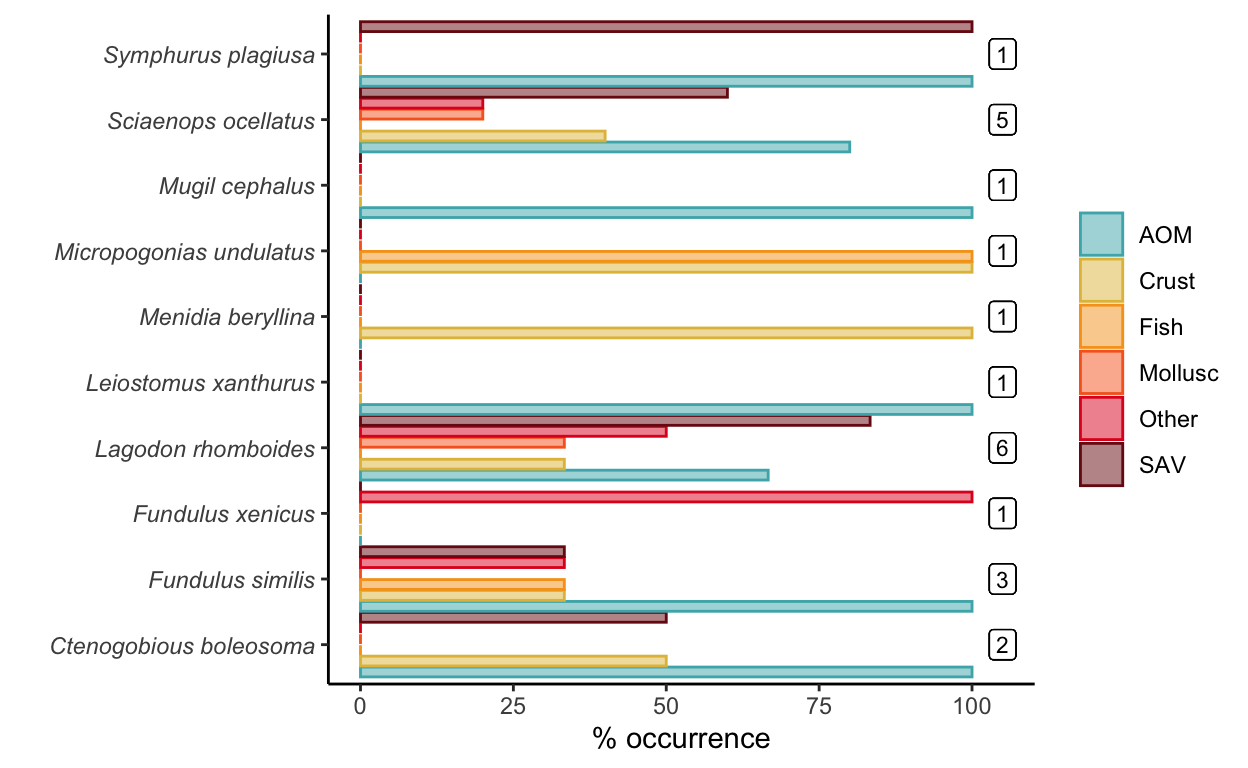
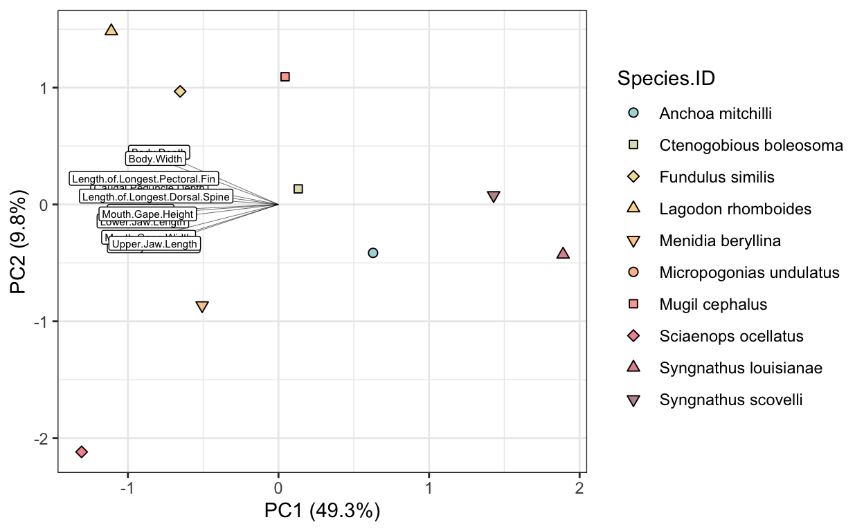
- Read in the morphometrics dataset. Then perform the following actions:
• for each individual, standardize the morphological measurements (columns 8 - 18) based on the total length by taking the ratio of the trait and TL.
• summarize the standardized morphological traits for each species by taking the mean across individuals.
• run a PCA on the morphological traits to examine morphological variation across fish species, makign sure that you plot the vectors alongside your species.
# morphometrics

morph <- read.csv(file = "data/fish_lab/morphometrics.csv")

morph.standardized <- morph %>%
  pivot_longer(cols = 8:18, names_to = "trait", values_to = "measurement") %>%
  mutate(stand.measurement = measurement/Total.Length) %>%
  group_by(Species.ID, trait) %>%
  summarize(mean.measurement = mean(stand.measurement)) %>%
  pivot_wider(names_from = trait, values_from = mean.measurement)

morph.meta <- morph.standardized[1:7]

morph.raw <- morph.standardized[-1]

morph.pca <- rda(morph.raw, scale = T, center = T)
sum.morph.pca <- summary(morph.pca)

morph_scores <- as.data.frame(sum.morph.pca$sites) %>%
  bind_cols(morph.meta)

morph_vectors <- as.data.frame(sum.morph.pca$species) %>%
  mutate(vectors = rownames(.))

morph_hulls <- morph_scores %>%
  group_by(Species.ID) %>%
  slice(chull(PC1, PC2))

morph.plot <- ggplot() +
  geom_point(data = morph_scores, aes(x = PC1, y = PC2, fill = Species.ID, shape = Species.ID), size = 2) +
  geom_segment(data = morph_vectors, aes(x = 0, xend = PC1,
                                        y = 0, yend = PC2), lwd = 0.1) +
  geom_label(data = morph_vectors, aes(x = PC1, y = PC2, label = vectors), size = 2) +
  scale_fill_fish_d(option = "Trimma_lantana", alpha = 0.5) +
  scale_color_fish_d(option = "Trimma_lantana") +
  theme_bw() +
  scale_shape_manual(values = rep(21:25, 2)) +
  xlab("PC1 (49.3%)") +
  ylab("PC2 (9.8%)")
morph.plot